Unit 7 - Graphs

Table of Contents

1. Overview: Graphs
2. Graph Applications
3. Breadth-First Search
4. Depth-First Search
5. Generalized Depth-First Search

7.1. Overview - Graphs

We've been studying trees for a bit now, which is one way of connecting related bits of data to each other. The parent-child relationship is a pretty intuitive one, and our binary tree, in which each parent can have a left and right child, is useful for a number of problem-solving situations.

Trees are actually a specialized form of a more generic way of describing data and the connections between them: the graph.

Graphs can be a bit more complicated than trees, but it's worth the trouble, because graphs can be constructed to help us solve all sorts of interesting problems.

7.1.1. Vocabulary

There are a few simple terms that we'll use in discussing graphs.

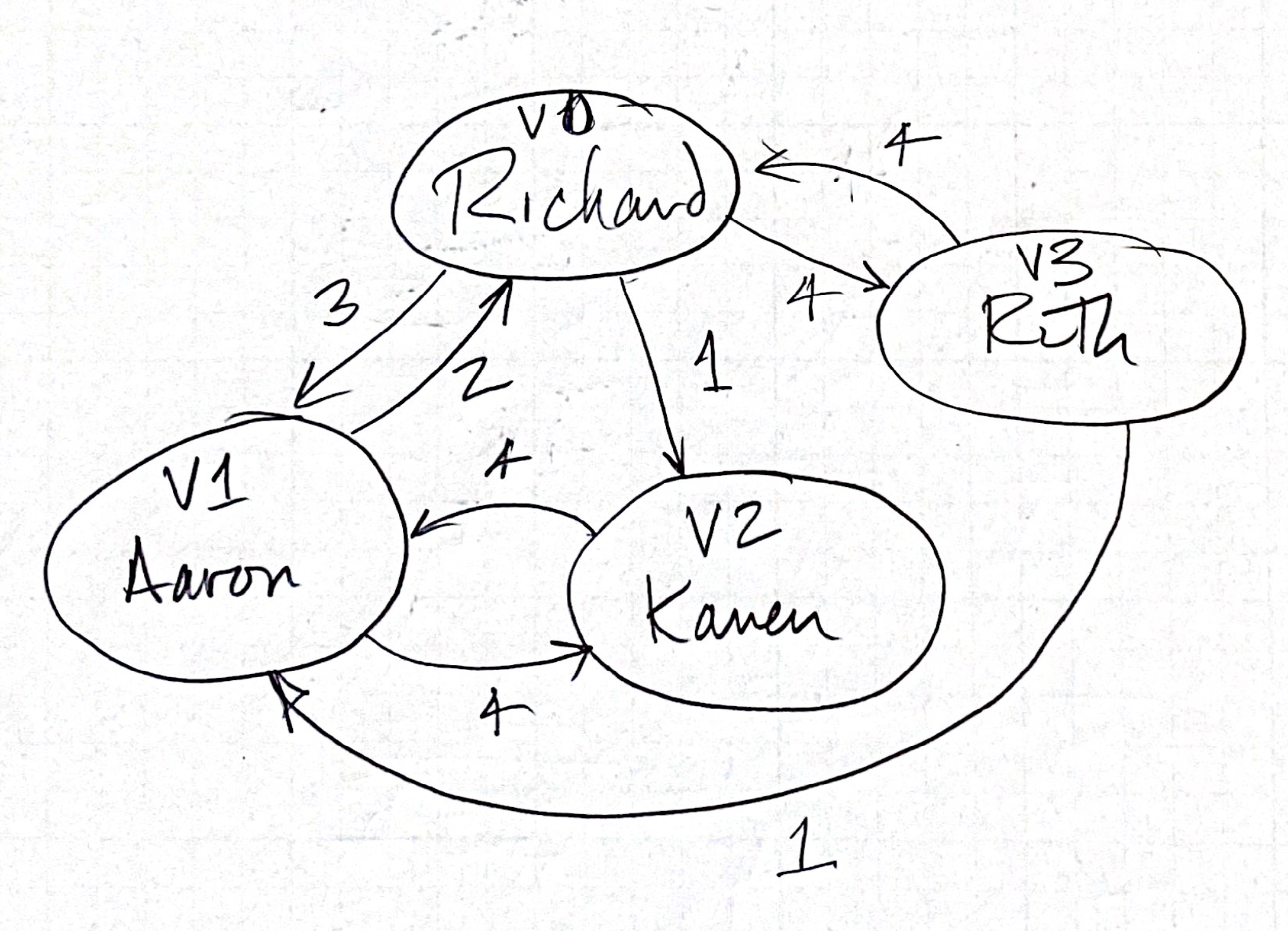
In the example shown here, relationships between Richard, Ruth, and their friends Aaron and Karen are represented by a graph with the weight of those relationships indicated.

7.1.2. The Graph Abstract Data Type

We'll have a number ways of interacting with our Graph. First let's define the Abstract Data Type, then we'll take a look at a way we can implement the ADT in Python.

7.1.3. Implementing the Graph ADT in Python

Although one can use a sparse array to represent the vertices and edges in a graph, we're going to use an "Adjacency List" to represent our graphs. In this strategy:

1. A Graph object keeps track of a list of Vertex objects and the edges that connect them.
2. Each Vertex object keeps track of the other vertices it's connected to, as well as the weight of those connections.

Graphs are made up of connections between vertices, so before we develop our Graph class, let's develop a Vertex class.

7.1.3.1. The Vertex class

Let's start with the Vertex first.

#!/usr/bin/env python3
"""
vertex.py
Describes the Vertex class
"""

class Vertex(object):
    """Describes a vertex object in terms of a "key" and a
    dictionary that indicates edges to neighboring vertices with
    a specified weight.
    """
    def __init__(self, key):
        """Constructs a vertex with a key value and an empty dictionary 
        in which we'll store other vertices to which this vertex is connected.
        """
        self.key = key
        self.neighbors = {}   # empty dictionary for neighboring vertices
    
    def set_neighbor(self, other, weight=0):
        """Adds a reference to a neighboring Vertex object to the dictionary, 
        to which this vertex is connected by an edge. If a weight is not indicated, 
        default weight is 0.
        """
        self.neighbors[other] = weight
    
    def __repr__(self):
        """Returns a representation of the vertex and its neighbors, suitable for 
        printing. Check out the example of 'list comprehension' here!
        """
        return f"Vertex({self.key}"
        
    def __str__(self):
        return ( f"{self.key} connected to: "
        + f"{[x.key for x in self.neighbors]}")
    
    def get_neighbors(self):
        return self.neighbors.keys()
    
    def get_key(self):
        return self.key
    
    def get_neighbor(self, other):
        """Returns the weight of an edge connecting this vertex with another,
        or None if the neighbor doesn't exist
        """
        return self.neighbors.get(other, None)

Once the Vertex class is written we can create two vertexes connected to each other:

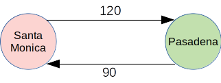
v1 = Vertex("Pasadena")
v2 = Vertex("Santa Monica")
v1.set_neighbor(v2, 90)
v2.set_neighbor(v1, 120)

This very simple graph be a way of representing how much time it takes for me to commute from one community to the other, with the weight representing a travel time in minutes. A physical representation of the graph might be something like this:

v1 = Vertex("Richard")
v2 = Vertex("Susie")
v3 = Vertex("Wayne")
v1.set_neighbor(v2)
v1.set_neighbor(v3, 4)
v2.set_neighbor(v3)
v2.set_neighbor(v1, 3)

Richard connected_to: ['Susie', 'Wayne']
Susie connected_to: ['Wayne', 'Richard']
Wayne connected_to: []

7.1.3.2. The Graph class

Our Vertex class has been designed so that each vertex knows who its neighbors are, but the Graph class will have methods that allow us to manage those vertices and their connections.

#!/usr/bin/env python3
"""Implements a graph of vertices"""
                        
from vertex import Vertex

class Graph(object):
    """Describes the Graph class, which is primarily a dictionary
    mapping vertex names to Vertex objects, along with a few methods
    that can be used to manipulate them.
    """
    def __init__(self):
        self.vertices = {}

    def set_vertex(self, key):
        self.vertices[key] = Vertex(key)

    def get_vertex(self, key):
        """Looks for the key in the dictionary of Vertex objects, and
        returns the Vertex if found. Otherwise, returns None.
        """
        '''
        # This is the classic way of doing that
        if key in self.graph.keys():
            return self.graph[key]
        else:
            return None
        '''
        # Single-line alternative
        return self.vertices.get(key, None)

    def __contains__(self, key):
        """This 'dunder' expression is written so we can use Python's "in"
        operation: If the parameter 'key' is in the dictionary of vertices,
        the value of "key in my_graph" will be True, otherwise False.
        """
        return key in self.vertices

    def add_edge(self, from_vert, to_vert, weight=0):
        """Adds an edge connecting two vertices (specified by key
        parameters) by modifying those vertex objects. Note that
        the weight can be specified as well, but if one isn't
        specified, the value of weight will be the default value
        of 0.
        """
        # if the from_key doesn't yet have a vertex, create it
        if from_vert not in self.vertices:
            self.set_vertex(from_vert)
        # if the to_key doesn't yet have a vertex, create it
        if to_vert not in self.vertices:
            self.set_vertex(to_vert)
        # now we can create the edge between the two
        self.vertices[from_vert].set_neighbor(self.vertices[to_vert], weight)

    def get_vertices(self):
        return self.vertices.keys()

    def __iter__(self):
        """Another 'dunder' expression that allows us to iterate through
        the list of vertices.
        Example use:
        for vertex in graph:  # Python understands this now!
            print(vertex)
        """
        return iter(self.vertices.values())

def main():
    g = Graph()
    g.add_edge("V0", "V1", 2)
    g.set_vertex("V2")
    g.add_edge("V0","V2",12)
    g.add_edge("V1", "V0", 3)
    for vertex in g:
        print(vertex)

if __name__ == "__main__":
    main()

What would the output be for this main program?

7.2. Overview - Graph Applications

Now that we have Graph and Vertex classes set up, let's see if we can use them.

We'll see how those two processes work in a variety of contexts.

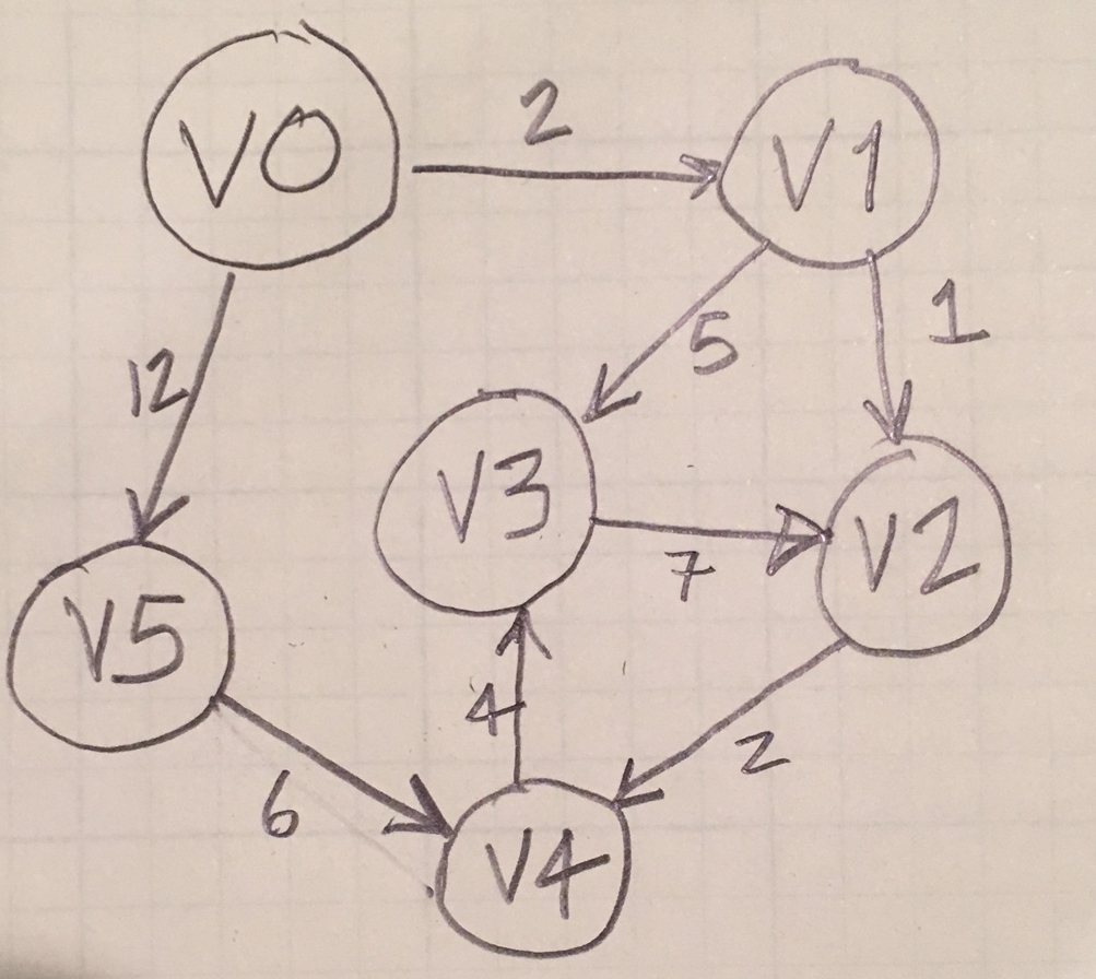
Warm-up: Create this Graph

Write a main() program that creates this graph and prints out its Python representation.

Show/hide the program

def main():
    g = Graph()             # Create an empty graph
    for i in range(6):      # Create a series of empty vertices with
        g.add_vertex(i)      # simple keys (the numbers 0-5)
    
    g.add_edge(0,1,2)        # Start adding edges connecting the vertices
    g.add_edge(0,5,12)
    g.add_edge(1,2,1)
    g.add_edge(1,3,5)
    g.add_edge(3,2,7)
    g.add_edge(2,4,2)
    g.add_edge(4,3,4)
    g.add_edge(5,4,6)
    
    # Here's one way of printing out the Graph
    # This is possible because we implemented __iter__
    for v in g:
        print(v)
    print("\n--------------\n")

if __name__ == "__main__":
    main()

7.3. Breadth-first Search (BFS)

We have the ability to create a directed graph now, which consists of edges (possibly weighted) connecting Vertex objects.

Once the graph has been constructed, there are two common algorithms for moving through the a graph:

1. performing a breadth-first search across the vertices, in which all of a given vertex's connections are explored before descending further down into the graph
2. performing a depth-first search through a series of connected vertices, exploring a chain of connected vertices to the end before coming back to the next connection

Which search strategy you employ depends upon the problem you are trying to solve.

7.3.1. Enhancing the Vertex class

It will be necessary for us to keep track of vertices that we've already explored (perhaps by arriving at them from a previous path), so we'll keep track of the state of every node as either "unexplored", "being explored", or "fully explored". It's common to consider the nodes as having a virtual color to identify these states: perhaps using a "white" node for unexplored, "gray" for being explored, and "black" for fully explored.

It will also be helpful to keep track of distances traveled as we traverse the graph, so we'll include instance variables for tracking that as well.

Finally, as we explore a vertex it will become advantageous for us to have a "Back button" that allows us to backtrack to the preceding vertex (without having to use a stack).

Let's modify the Vertex class to accommodate these new features:

class Vertex(object):
    """Improves the vertex class to include not only a key and neighbors,
    but also a "color" (used to identify exploration state), a "distance"
    (used by some algorithms to measure number of vertices traversed), and
    "previous", a convenient pointer to a previous vertex in a path.
    Note also that the "weight" to a neighbor is coded as a value in a
    key-value pair in the `neighbors` dictionary.
    """
    def __init__(self, key):
        """Constructs a vertex with a key value and an empty dictionary 
        in which we'll store other vertices to which this vertex is connected.
        """
        self.key = key
        self.neighbors = {}   # empty dictionary for neighboring vertices
        self.color = 'white'
        self.distance = 0
        self.previous = None
    
    def set_neighbor(self, other, weight=0):
        """Adds a reference to a neighboring Vertex object to the dictionary, 
        to which this vertex is connected by an edge. If a weight is not indicated, 
        default weight is 0.
        """
        self.neighbors[other] = weight
    
    def get_color(self):
        return self.color
    
    def set_color(self, color):
        self.color = color
    
    def get_distance(self):
        return self.distance
    
    def set_distance(self, new_distance):
        self.distance = new_distance
    
    def get_previous(self):
        return self.previous
    
    def set_previous(self, new_prev):
        self.previous = new_prev
    
    def __repr__(self):
        """Returns a representation of the vertex and its neighbors, suitable for 
        printing. Check out the example of 'list comprehension' here!
        """
        return f"Vertex({self.key}"
        
    def __str__(self):
        return ( f"{self.key} connected to: "
        + f"{[x.key for x in self.neighbors]}")
    
    def get_neighbors(self):
        return self.neighbors.keys()
    
    def get_key(self):
        return self.key
    
    def get_neighbor(self, other):
        """Returns the weight of an edge connecting this vertex with another,
        or None if the neighbor doesn't exist
        """
        return self.neighbors.get(other, None)

7.3.2. The Word Ladder Game

Here, we'll use a breadth-first search (BFS) to solve the Word-Ladder problem.

BEAR
BOAR
BOOR
.
.
.

To solve a Word Ladder problem algorithmically, we will:

1. create a graph of words that are related to each other according to the rules of the game: each word will be a vertex that is connected to other words that vary from the original by a single letter
2. Then we can follow a path from one word to another to identify a solution

How are we going to create the graph of words, though?

7.3.2. Building Graph of Related Words

There are a variety of strategies that we might use to identify words that are connected to each other.

One strategy would be to begin with a word, and then check every other word in the word list to see if it differs by one letter. For every word that matches that description, we'd need to then go through every word again to find those that differ by one letter.

def build_graph():
    g = Graph()
    infile = open('three-letter_words.txt', 'r')
    # create vertices
    for line in infile:
        word = line.rstrip()
        g.set_vertex(word)
    infile.close()
    # connect vertices that are off by one letter
    for v1 in g:
        for v2 in g:
            if off_by_exactly_one(v1.get_key(), v2.get_key()):
                g.add_edge(v1.get_key(), v2.get_key())
    
    return g

7.3.4. Breadth-First Searching

A graph connecting all the words that differ from each other by one letter might start out looking something like this:

ACT connected to: ['ANT', 'ART']
ANT connected to: ['ACT', 'ART']
ART connected to: ['ACT', 'ANT']
TAT connected to: ['TAR', 'PAT', 'TAP', 'TAN']
TAR connected to: ['TAT', 'CAR', 'TAP', 'TAN']
CAR connected to: ['TAR', 'CAB', 'CAN', 'CAP']
CAB connected to: ['CAR', 'CAN', 'CAP']
CAN connected to: ['CAR', 'CAB', 'RAN', 'PAN', 'TAN', 'CAP']
RAN connected to: ['CAN', 'PAN', 'TAN']
PAN connected to: ['CAN', 'RAN', 'PAT', 'TAN', 'PEN']
PAT connected to: ['TAT', 'PAN']
TAP connected to: ['TAT', 'TAR', 'TAN', 'NAP', 'LAP', 'CAP']
TAN connected to: ['TAT', 'TAR', 'CAN', 'RAN', 'PAN', 'TAP', 'TEN']
TEN connected to: ['TAN', 'YEN', 'KEN', 'PEN']
NET connected to: []
YEN connected to: ['TEN', 'KEN', 'PEN']
KEN connected to: ['TEN', 'YEN', 'PEN']
PEN connected to: ['PAN', 'TEN', 'YEN', 'KEN']
NAP connected to: ['TAP', 'LAP', 'CAP']
LAP connected to: ['TAP', 'NAP', 'CAP']
CAP connected to: ['CAR', 'CAB', 'CAN', 'TAP', 'NAP', 'LAP']

Now how do we go about looking through that graph to find the path we want?

7.3.5. Implementing the breadth-first search

With the extended version of the Vertex class we can implement a Breadth-First Search algorithm.

def bfs(g, start):
    """Goes through the vertices to create a set of predecessor links
    between the vertices (in addition to the edges that are already 
    there
    """
    start.set_distance(0)
    start.set_previous(None)
    current = start
    q = Queue()
    print("Putting",current.get_key(),"on the queue")
    q.enqueue(current)
    while not q.is_empty():
        current = q.dequeue()
        print("Just pulled",current.__repr__(),"off the queue!")
        for neighbor in current.get_neighbors():
            # if we haven't seen this neighbor yet
            if neighbor.get_color() == 'white':
                print("Processing",neighbor.get_key(),"by setting color to gray")
                neighbor.set_color('gray')
                neighbor.set_distance(current.get_distance() + 1)
                neighbor.set_previous(current)
                print("Adding",neighbor.__repr__(),"to the queue")
                q.enqueue(neighbor)
                print("Current queue:",q)
                input("[Enter] to continue...")
            elif neighbor.get_color() == 'gray':
                print("Found a gray neighbor",neighbor.get_key(),". It's already in the queue.")
            else:
                print("Found a black neighbor", neighbor.get_key(),"that's already been processed.")
        print("Finished processing",current.get_key())
        print("Setting it to black")
        current.set_color('black') 
        input("[Enter] to continue")

You'll understand this algorithm much better if you take a moment to trace through a sample graph.

7.3.5. Traversing the Graph

Finally, once the breadth-first search has been performed, the graph will have the important vertices identified with a non-None predecessor. We can traverse the graph from any valid vertex in the graph to get back to the starting position, identifying the complete path along the way.

def traverse(g, start, finish):
    """Works backwards from the finish vertex, following `previous` vectors
    all the way to the start.
    """
    if finish != None:
        current = finish
        while current.get_previous() != None:
            print(current.get_key(), current.get_distance())
            current = current.get_previous()
        if current == start:
            print(current.get_key()) # The last ie. first item in the path
        else:
            print("Couldn't find a path!")
    else:
        print("Finishing vertex doesn't exist!")

Run a few experiments to see how the algorithm works. Put some print statements in the program to get a better idea of what's going on.

What happens when there isn't a path from one work to another? How could you modify the program to handle that issue?

Are their modifications that would make the program better? Is there a way to print out the ladder first-to-last rather than last-to-first?

7.3.6. Optimizing

This has been a nice little activity up to this point, but we're going to run into a problem. Take this list of four-letters and put build a graph based on them, where vertices of words that are "off-by-one-letter" share an edge.

What do you observe?

Here's a different strategy suggested in our book:

1. Create an empty dictionary
2. Take a word of a given length: "LION" for example
3. Go through that removing a single letter each time: "_ION", "L_ON", "LI_N", "LIO_"
4. For each of those "letter-removed" values, create an entry in the dictionary. The associated value for the key "_ION", for example, will have a list of words that fit that pattern: ["CION","LION","PION"].
5. Once all of the words have been identified in the list for that pattern, create a Vertex for each word and connect them in the Graph with an edge.

How is this helpful? The "letter-removed" dictionary act as an intermediary data structure, vastly reducing the number of the n-squared words that need to be compared with each other.

Here's the code that will do that:

def build_graph(word_file):
    """Builds a graph of related 4-letter words"""
    buckets = {}  # each "bucket" is a "3-letter + _" entry that
                  # contains the actual 4-letter words that
                  # correspond to that pattern
    g = Graph()   # connects all the entries in the bucket
    infile = open(word_file,'r')
    # create buckets of words that differ by one letter
    for line in infile:
        word = line.rstrip() # remove newline character if there is one
        for i in range(len(word)):
            # replace one letter in the word by a _
            key = word[:i] + '_' + word[i+1:]
            if key in buckets:       # if we already have pattern
                buckets[key].append(word)  # add this word to it
            else:
                buckets[key] = [word]      # create a new bucket
                                           # with this word in it
    
    # Now build the graph, with vertices and edges for words in
    # the same bucket
    for key in buckets.keys():
        for word1 in buckets[key]:
            for word2 in buckets[key]:
                if word1 != word2:
                    g.add_edge(word1,word2)
    return g

Of course we need to get a list of four-letter words that this method can work on. Perhaps begin with this short list that's useful for development purposes, and then later on, get this long list of words.

Take a moment to see if you can get build_graph() working. Add some print statements that will allow you to see what's happening behind the scenes.

7.4. Depth First Searching

In the previous example, we looked through the graph one level at a time, cataloging each level of vertices in the graph as we proceeded, looking for a path of vertices that would provide a solution for us.

This breadth-first search strategy is appropriate for some types of problems. Others are better solved using a depth-first search strategy, in which valid paths are pursued to the end as they are encountered.

Let's see how that works.

7.4.1. The Knight's Tour Problem

A knight in chess is able to move in its odd L-shaped pattern, 2 steps in one direction and 1 more step either to the left or right from that direction. A "tour" of the knight is one in which is manages to visit every single location in a square range of locations.

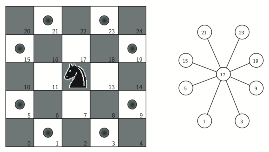
A knight on square 12 has legal moves as shown. Picture from Miller and Ranum's Problem Solving with Algorithms and Data Structures using Python.

We'll begin our solution by creating a graph of the possible moves of the knight. Then we'll perform a depth-first search of that graph to produce a solution.

7.4.2. Creating a graph of the Knight's possible moves

In our graph, each position on the board will be represented by a vertex, and each edge between those vertices will represent a move of the knight.

def create_knight_graph(board_dimension):
    """Sets up a graph of legal knight moves on a board of a given
    size.
    """
    g = Graph()
    for row in range(board_dimension):
        for col in range(board_dimension):
            
            # calculate a nodeID using row and column
            # standard strategy for converting x-y values to
            # a single value
            nodeID = row * board_dimension + col
            
            # get the legal moves from here and store them in 
            # a list
            next_moves = find_legal_moves(row, col, board_dimension)
            for move in next_moves:
                moveID = move[0] * board_dimension + move[1]
                g.add_edge(nodeID, moveID)
    return g

The question of how to find those legal moves is relatively easy to solve.

def find_legal_moves(row, col, dimension):
    """Returns a list of row-col locations that:
        a) follow a knight's move ("up, up, over"), and
        b) are still on the board
    """
    legal_moves = []
    
    # describe offsets by row, col
    offsets = ( (2, 1), (2, -1), (-2, 1), (-2, -1), 
                (1, 2), (1, -2), (-1, 2), (-1, -2))
    
    for offset in offsets:
        r = row + offset[0]
        c = col + offset[1]
        if is_legal(r, dimension) and is_legal(c, dimension):
            legal_moves.append((r, c))
    return legal_moves
        
def is_legal(value, dimension):
    """Checks to see if the value is on the board (between 0 inclusive
    and dimension exclusive)
    """
    return value >= 0 and value < dimension

Okay, with these sections of code written, we have a graph with all of the possible knight positions, and edges connecting each of those positions with a legal move to another position.

One interesting thing we can do is view that graph.

7.4.3. Performing the tour with a depth-first search

def dfs(depth, vertex_path, current, limit):
    """Performs a recursive depth-first search, returning True if the depth
    reaches the limit, otherwise False.
    * `depth` tracks how far we are in the search, and is incremented with each
      recursive call
    * `vertex_path` is a list that is used as a stack to accumulate vertices
      that are part of the path
    * `current` identifies the current vertex being examined
    * `limit` an integer that indicates how many vertices we need to traverse
      to succeed
    """
    current.set_color('gray')
    
    # Add this (potentially successful?) vertex to the end of the path
    vertex_path.append(current)
    
    # Go through all the neighbors for this vertex, and investigate each one
    # by calling dfs on it!
    if depth < limit:       # we haven't gotten all the squares
        neighbor_list = list(current.get_neighbors())
        i = 0
        done = False
        while i < len(neighbor_list) and not done:
    
            # This is the dfs part. Dig down into the neighbors and go as far as you
            # can with each one before coming back to check out the next neighbor.
            if neighbor_list[i].get_color() == 'white':     # haven't been here yet
                done = dfs(depth + 1, vertex_path, neighbor_list[i], limit)
            i += 1
        # We've gone through all the possibilities and haven't finished so we're 
        # going to have to backtrack. That means popping this current vertex off the
        # path, and also resetting its color to "white", so it can potentially be 
        # explored again by a later search.
        if not done: 
            vertex_path.pop()
            current.set_color("white")
    else:
        done = True
    return done

And now, all that's left to do is to initialize the board and initiate the search for a solution.

def main():
    '''
    g = create_knight_graph(5)
    for v in g:
        print(v)
    '''

    DIM = 5    # 8x8 chessboard
    g = create_knight_graph(DIM)

    # vertex_path will return the final solution
    vertex_path = []

    # Specify which vertex to begin from: 
    #
    #                    Columns
    #               0    1    2    3
    #            +-------------------+
    #        0   |  0 |  1 |  2 |  3 |
    #            +-------------------+
    #        1   |  4 |  5 |  6 |  7 |
    #  Rows      +-------------------+
    #        2   |  8 |  9 | 10 | 11 |
    #            +-------------------+
    #        3   | 12 | 13 | 14 | 15 |
    #            +-------------------+

    # Specify where to begin tour from
    start_vertex = g.get_vertex(0)
    start_time = time.time()
    # initiate search, with empty path to begin with,
    # initial position specified, and a final distance
    # provided.
    dfs(0, vertex_path, start_vertex, DIM*DIM - 1)
    stop_time = time.time()
    print("Searching finished")

    # Display solution
    if len(vertex_path) == 0:
        print("No solution found")
    else: 
        print([vertex.key for vertex in vertex_path])
    print("Elapsed time: " + str(stop_time - start_time) + " seconds")

if __name__ == "__main__":
    main()

Recursively searching solutions on an 8x8 chessboard might take a while. If you get tired of waiting for your program to finish, you might try running a smaller chessboard (6x6?) and seeing if that will finish in a more reasonable amount of time.

It's interesting to view the search as it takes place. In the dfs function, right after the vertex current is appended to the vertex_path, included the following lines:

# Print the path to this point
os.system("clear")
print([vertex.get_key() for vertex in vertex_path])

Having to print significantly slows down the recursion process, however, so you probably don't want to leave this code in there. Comment it out after you're done investigating.

7.4.4. Improving the depth-first search with a heuristic

The graph of possible moves is static—it describes all the possible moves between vertices, and there are no improvements to make there.

But we can improve the performance of the search by programming additional consideration into the traversal. For example, which position is it easier to find a legal move from, near the middle of the board or near the edge of the board?

The edge of the board has fewer possibilities, so perhaps it makes sense to try moving through those locations first, leaving the positions at the middle of the board for later on when they'll be more likely to have a move available.

neighbor_list = list(current.get_neighbors())

neighbor_list = list(order_by_avail(current))

def order_by_avail(vertex):
    """What's going on in here?!
    This fancy method takes a vertex, looks at its neighbors,
    and identifies which of them have the *fewest* possible
    moves from there. By choosing to move to a neighbor with
    fewer possibilities *now*, we'll leave more flexibility
    for our next vertex choices later on.
    
    Getting this heuristic to work requires some interesting
    coding!
    """
    neighbor_list = []       # Will store both the neighbor
                            # and how many neighbors they
                            # have, as a tuple
    for neighbor in vertex.get_neighbors():
        if neighbor.get_color() == 'white':   # available
            c = 0           # counter for THIS neighbor
            for w in neighbor.get_neighbors():
                if w.get_color() == 'white':
                    c = c + 1   
            neighbor_list.append((c,neighbor))
    # We now have a list of (count, neighbor) values
    # We want to order them by count, from low to high
    neighbor_list.sort(key=lambda x: x[0])
    # Now, send back a list of the neighbors that have
    # been ordered as needed
    return [neighbor[1] for neighbor in neighbor_list]

How does this affect our search times?

(base) rwhite@Ligne2 knights_tour % python knights_tour.py
Done!
[1, 18, 35, 52, 37, 54, 39, 22, 7, 13, 30, 47, 62, 45, 60, 43, 58, 41, 56, 50, 
33, 48, 42, 59, 44, 61, 55, 38, 28, 11, 26, 32, 49, 34, 24, 9, 3, 20, 5, 15, 21, 
6, 23, 29, 19, 4, 14, 31, 46, 63, 53, 36, 51, 57, 40, 25, 8, 2, 12, 27, 17, 0, 
10, 16]
Elapsed time: 927.4193122386932 seconds
(base) rwhite@Ligne2 knights_tour % python knights_tour_improved.py
Done!
[1, 16, 33, 48, 58, 41, 56, 50, 60, 54, 39, 22, 7, 13, 23, 6, 12, 2, 8, 18, 3, 
9, 24, 34, 40, 57, 51, 61, 55, 38, 44, 59, 49, 32, 17, 0, 10, 27, 42, 25, 19, 4, 
14, 29, 35, 52, 62, 45, 28, 43, 26, 11, 5, 20, 37, 47, 30, 15, 21, 31, 46, 63, 
53, 36]
Elapsed time: 0.00043702125549316406 seconds
(base) rwhite@Ligne2 knights_tour %

7.4.5. Rectangular boards

A related topic of interest is the knight's tour on a rectangular shaped board.

Modify your programs so that they work with a given number of rows and columns, where rows <= cols.

Only certain types of rectangular boards are able to be solved. See if you can identify which boards offer a solution and which don't.

7.5. Generalized Depth-First Search

The Knight's Tour analysis involved creating a graph of connected nodes, and then designing an algorithm that would look for a single, non-branching path through that graph to identify the steps in the tour.

There are other strategies we can use to analyze a graph, including looking at every single connection ("edge") between every single vertex (node) in the graph. This has the potential to create not just a single tree of interconnected nodes, but a "forest" of trees connecting nodes.

For our next applications (following our textbook), we're going to create a new class called DFSGraph which inherits from Graph, and includes a new instance variable and two new methods (in addition to the ones it inherits):

class DFSGraph(Graph):
    """Used to create a depth first forest. Inherits from the
    Graph class, but also adds a `time` variable used to track
    distances along the graph, as well as the two methods below.
    """
    
    def __init__(self):
        super().__init__()
        self.time = 0       # allows us to keep track of times when vertices
                            # are "discovered"
    
    def dfs(self):
        """Keeps track of time (ie. depth) across calls to dfsvisit
        for *all* nodes, not just a single node: we want to make sure
        that all nodes are considered, and that no vertices are left
        out of the forest.
        """
        for aVertex in self:             # iterate over all vertices
            aVertex.set_color('white')   # initial value of unexamined vertex
            aVertex.set_pred(-1)         # no predecessor for first vertex
        for aVertex in self:             # now start working our way through
            if aVertex.get_color() == 'white':   # a depth-first exploration
                self.dfsvisit(aVertex)           # of the vertices
    
    def dfsvisit(self, start_vertex):
        """Effectively uses a stack (by calling itself recursively) to
        explore down through the depth of the graph.
        """
        start_vertex.set_color('gray')          # Gray color indicates that this
                                                # vertex is the one being explored
        self.time += 1                          # Increment the timer
        start_vertex.set_discovery(self.time)   # Record the current time for this 
                                                # vertex's discovery
        for next_vertex in start_vertex.get_connections():  # check all connections
            if next_vertex.get_color() == 'white':          # if we've touched this
                next_vertex.set_pred(start_vertex)          # reset pred to our start
                self.dfsvisit(next_vertex)                  # continue depth search
        start_vertex.set_color('black')         # After exploring all the way down
        self.time += 1                          # Last increment
        start_vertex.set_finish(self.time)      # Stop "timing"

Recall that the Graph class, from which DFSGraph inherits, already has methods that we can use to add vertices and edges to a graph.

Once we've done that, we can call dfs() to create the depth-first relationships for the graph. The dfs() method itself calls the helper method dvsvisit() to establish those relationships.

Use the example in the next section to develop an understanding of how these relationships are developed.

7.5.1. A small graph

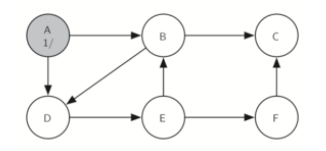
Before we apply the DFSGraph to an actual problem, let's see how to set up a small DFS graph.

Write a small program that

1. Creates a DFSGraph
2. Adds the vertices/edges from the graph shown here
3. Calls the dfs() method to create a graph of the vertices
4. Prints out all the vertices so what we can see how they're connected

#!/usr/bin/env python3
"""
book_example.py
"""

from atds import *

def main():
    # Set up graph
    g = DFSGraph()
    # Add all the edges (vertices are created in method)
    g.add_edge('A','B')
    g.add_edge('A','D')
    g.add_edge('B','D')
    g.add_edge('B','C')
    g.add_edge('D','E')
    g.add_edge('E','B')
    g.add_edge('E','F')
    g.add_edge('F','C')
    # Explore the graph using the depth-first search, establishing
    # vertex relationships in the process
    g.dfs()
    # Print out the resulting vertices in the graph
    for v in g:
        print(v, "\n")

if __name__ == "__main__":
    main()

7.5.2. Making Pancakes (Topological Sorting)

Follow the instructions outlined in our textbook to create a recipe for making pancakes. :)

#!/usr/bin/env python3
"""
pancakes.py
"""

from atds import Vertex, Graph, DFSGraph

def main():
    g = DFSGraph()
    
    # Describe all the edges as a large tuple of tuple-pairs
    edges = (("3/4 cup milk","1 cup mix"),
             ("1 egg", "1 cup mix"),
             ("1 Tbl Oil", "1 cup mix"),
             ("1 cup mix", "heat syrup"),
             ("heat syrup", "eat"),
             ("heat griddle", "pour 1/4 cup"),
             ("1 cup mix", "pour 1/4 cup"),
             ("pour 1/4 cup", "turn when bubbly"),
             ("turn when bubbly", "eat"))
    
    # Put all the edges in the graph
    for edge in edges:
        g.add_edge(edge[0],edge[1])
    
    # Create the forest
    g.dfs()
    
    # Put all the vertices in a list:
    vertex_list = [g.get_vertex(k) for k in g.getVertices()]
    
    # Sort the vertices by finish time to create the recipe list
    vertex_list.sort(key=lambda x: x.getFinish())
    vertex_list.reverse()
    
    # Print recipe steps
    print("Here's how to make pancakes")
    for step in vertex_list:
        print(step.get_key())

    
if __name__ == "__main__":
    main()