Unit 5 - Sorting, Searching, and Hashing
Table of Contents
5.1. Overview - Sorting, Searching, and Hashing
In this unit we're going to take a look at some classic algorithms and data structures.
Sorting algorithms work on collections of related data items and sort them according to some criteria. Because the criteria is arbitrary and because we're focused on the sorting process itself (rather than what type of data we're sorting), our examples here will typically work on collections of integers.
We'll be sorting lists of integers.
There are lots of different strategies for sorting data. It's interesting to think about how that might happen, what systems or strategies there are for doing that kind of thing.
How do you sort?
If someone gives you a list of numbers written down, how do you go about putting the numbers in order?
If someone gives you a series of cards, how do you go about putting them in order?
If you have a roomful of people all born on different days of the year, how would you go about putting them in order of their birth date?
How would you give instructions to someone else to put any of these collections in order?
The topic of Searching through a collection of data is another interesting topic. There are pretty much only two commonsense ways of finding items in a collection, and which one you use depends on the way the collection is implemented, and whether or not the collection is ordered. We'll look at both of those possibilities.
Related to the question of searching is the fascinating topic of hashing.
Definition: Hashing
Hashing refers to the process of storing information in a data structure according to a function so that data values can be searched for in O(1) time.
A hash table is the table in which the data values are stored. The function that is used to store and retrieve items in the table is called the hash function.
We'll soon learn all about it!
5.2. Sorting
The process of sorting is already familiar to you. In your previous Computer Science course you learned about the Selection Sort, for example:
Selection Sort
The Selection Sort algorithm works as follows:
- Begin with a list of unsorted items.
- Beginning with the first item on the list, go through and find the location of the smallest value in the list.
- After finding the location of the smallest value, exchange the value at that smallest location with the value at the start of the list. (Smallest value on list is now first in the list.)
- Repeat, starting at 2nd position: go through list, find location of smallest item on list, and place it in 2nd position.
- Go through entire list in this fashion until done.
What does this look like?
Selection Sort Example
Take a moment to perform a Selection Sort by hand on this list of numbers. Go through the list, write down important values, and write a new list underneath the old one each time values in the list are changed.
List to sort: 11 9 17 5 12
Now let's implement a Selection Sort in Python.
Selection Sort
Complete the methods in the program below to implement a Python-based version of Selection Sort.
#!/usr/bin/env python3
"""
selection_sort.py
Creates a list of random values and sorts them using the
Selection Sort algorithm.
"""

import time
import random

def generate_random_numbers(length, range_of_values):
    """Generates a list of "length" integers randomly
    selected from the range 0 (inclusive) to
    range_of_values (exclusive) and returns it to
    the caller.
    """
    # write code here


def selection_sort(nums):
    """Takes the list "nums" and sorts it using the
    Selection Sort algorithm.
    """
    # write code here


def display(a_list):
    """Prints out the list "a_list" on the screen. To
    be used for debugging, or displaying the initial
    and final state of the list.
    """
    # write code here


def main():
    NUM_OF_VALUES = 10
    nums = generate_random_numbers(NUM_OF_VALUES, 1000)
    display(nums)
    start = time.time()
    selection_sort(nums)
    stop = time.time()
    display(nums)
    print("Sorted {0:10d} values, execution time: {1:10.5f} seconds".format(NUM_OF_VALUES, stop - start))

if __name__ == "__main__":
    main()
Once the sorting process is working, collect some data:
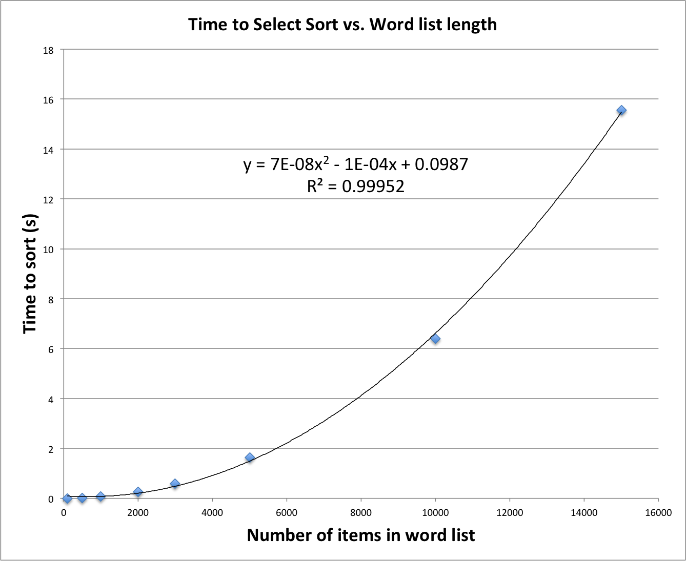
Graphically identifying the performance of the Selection Sort
Create a new version of your Selection Sort program that collects data for a range of data set sizes (length of the random number list), and then plot sort time (s) vs. size of data set (values) using a spreadsheet program.
Perform a regression on the data you've collected. Does it match the published Big-O value for the Selection Sort algorithm?
And once you've got that figured out...
Analyze the performance of the Selection Sort
Go through your Selection Sort algorithm to identify list accesses for an array of n elements. Based on your analysis of T(n), determine O(n).
How many times do we access an array element in Selection Sort?
- The size of the array =
n, and going through the array to find the smallest element = n accesses. - Swapping the two elements—
[smallest_loc]and[i]—costs us 2 accesses. - Now we have one less element to visit in the whole array = n-1 accesses.
- Swap two elements = 2 accesses...
So....
(n + 2)    +    (n-1 + 2)    +    (n-2 + 2)   +  ...  +  (2 + 2)

    [n + (n-1) + (n-2) +  ...  + 2]    +     [(n-1) * 2]
For the first part:
[2 +  ...  + n] =
    [sum of 1 to n] - 1 =
    n(n+1)/2        - 1     +    (n-1) * 2 (from the second part above)
Multiply out to get T(n) = n2/2 + 5n/2 - 3.
T(n) represents the Time (in "accesses") for the algorithm to run.
The "big-O notation" version of this polynomial is based on the largest order, the n2 term. Thus, we say "the Selection Sort algorithm runs in time n2."
5.2.1. Insertion Sort
The insertion sort is another strategy that can be used to sort a list of values.
Algorithm: Insertion Sort
The Insertion Sort takes a list of values and begins working through from left to right with a sublist of increasing size. The sublist consisting of only the first value is considered sorted.
Take the item to the right of that sublist, then, and move to the left, looking for the location where that item should be placed to maintain the sorted order of the list. As values are considered, they are moved over to the right, until the correct location is identified. Place this value at that location. The sublist is now one larger in size, but still sorted.
Continue with items to the right of the sublist until the entire list has been sorted.
Once you've developed an understanding of the Insertion Sort, implement a demonstration of that algorithm.
5.3. Searching
We're always storing data on the computer, and we're always trying to retrieve that data so that we can work with it, edit it, manipulate it, and display it. There are two classical means of searching for data that we've stored in a collection.
5.3.1. Linear Search
A linear search is just what it sounds like: given a list of values (sorted or unsorted), go through the list one item at a time, starting at the beginning, and checking each value in turn until you either:
- Find the item on the list, in which case you indicate its location, or
- You go through the entire list and don't find the number, in which case you indicate that the search term has not been found on the list.
A linear search is not usually the most efficient means of finding an item in a list, but it's a good start for us at this point.
Let's see how to write one.
linear_search.py
Write a program linear_search.py that uses a main() function to create a list of random integers. Then define a function search() that takes two parameters--a list of integers, and an integer to search for--and returns the position (index) of the number in the list, or a None if the number is not on the list.
| Search patterns to try | ||
| List to search | Item to look for | Expected result |
| [20, 3, 13, 4, 7, 9, 7, 14, 1] | 7 | 4 |
| [20, 3, 13, 4, 7, 9, 7, 14, 1] | 20 | 0 |
| [20, 3, 13, 4, 7, 9, 7, 14, 1] | 1 | 8 |
| [20, 3, 13, 4, 7, 9, 7, 14, 1] | -2 | None |
5.3.2. Binary Search
If your list of items has already been sorted according to some key—the value of the item, or the serial number of an item in inventory, or its location alphabetically—we can use a divide-and-conquer strategy to find an item in the sorted list.
Binary Search algorithm
The Binary Search algorithm works as follows:
- Begin with a list of sorted items and a "search item" that you're looking for.
- Compare the search item with the item at the middle of the sorted list.
- If the items match, you've found the location of that item!
- If the search item is greater than the middle item of the list, the bottom half of the sorted list can be eliminated from consideration. The top half of the list will become our new search space.
- If the search item is less than the middle of the list, the upper half can be eliminated, and the bottom half of the list will become our new search space.
- Continue searching through the smaller and smaller sections of lists until either the search item is found, or it is not found.
The Binary Search can be tricky to implement. Challenges include identifying the middle of a list of an even number of items, and keeping track of upper- and lower-bounds of the search space. Typically you'll want to have variables to track the lower index of the part of the list you're looking at, the upper part of the list, and the calculated middle of the list. Then adjust those values as you get closer and closer to finding the location of the search value.
There are also more sophisticated concerns, like "what happens if you have a billion items to search through?" Large lists like this can tax an algorithm, and even the experts can get tripped up.
We'll keep things simple in here.
Once you think you know how a binary search works, take a few moments to see if you can write and debug a Python version of it.
Write a Binary Search program
Write a program binary_search.py that:
- begins with this sorted list
l = [1, 2, 3, 4, 7, 9, 13, 14, 20] - asks for a search item
- calls a function
searchthat performs a Binary Search for that item in your list. That function will use a loop to examine successively smaller search spaces in the list. - The function should return the index of the item, or a -1 if not found.
- The main program should print the location (index) of the search item, if it exists. Otherwise, print out a "search item not found" message.
You will certainly find it handy to include some print() statements to reveal the progress of your search as it goes.
Test your program with the following lists to see if it works. When testing your program, be sure to look for an item that is on the list, and also an item that isn't on the list.
| to try | ||
| List to search | Item to look for | Expected result |
| [1, 2, 3, 4, 7, 9, 13, 14, 20] | 7 | 4 |
| [1, 2, 3, 4, 7, 9, 13, 14, 20] | 1 | 0 |
| [1, 2, 3, 4, 7, 9, 13, 14, 20] | 20 | 8 |
| [1, 2, 3, 4, 7, 9, 13, 14, 20] | -2 | None |
| [1, 2, 3, 4, 7, 9, 13, 14, 20] | 23 | None |
| [1, 2, 3, 4, 7, 9, 13, 14, 20] | 10 | None |
| [4, 7, 9, 13, 14, 20] | 9 | 2 |
| [4, 7, 9, 13, 14, 20] | 13 | 3 |
| [4, 7, 9, 13, 14, 20] | 20 | 5 |
| [4, 7, 9, 13, 14, 20] | 2 | None |
| [4, 7, 9, 13, 14, 20] | 10 | None |
| [4, 7, 9, 13, 14, 20] | 22 | None |
5.3.3. Binary Search, recursively
The version of the Binary Search above uses variables to keep track of the lower, upper, and middle indexes in the list, and manipulates those points to narrow the range of values being examine.
It may not surprise you that the binary search can be easily implemented using recursion: the search function, which examines a list with upper and lower bounds, can be used to call itself with changes in the upper and lower bounds, all the time reducing the search space.
Write a recursive Binary Search program
Write a program binary_search_recursive.py that:
- begins with this sorted list
l = [1, 2, 3, 4, 7, 9, 13, 14, 20] - asks for a search item
- calls a function
searchrecursively so that it performs a Binary Search for that item in your list. Thesearchfunction should include parametersarrfor the list of numbers,valuefor the search term,lowerfor the lower bound of the search space, andupperfor the upper bound of the search space. - Print out the location of the search item, if it exists. Otherwise, print out a "search item not found" message.
Test your binary_search_recursive.py with the same lists and values given above.
5.4. Hashing
Most introductory classes get a chance to touch on linear and binary searching. A third strategy for looking things up in a collection is a bit more sophisticated, and involves using a certain strategy when we first store the items in memory.
Let's take a look at hashing.
5.4.1. The Principles of Hashing
Just as a list allows us to store items for access later, a hash table allows us to store items for access later. In a list we access items according to their location in the list—their index—but in a hash table, we identify the item directly by its value.
The hash table has a series of slots for holding values. At any given time, some of those slots will be filled with values (our data), and some of them will be unfilled. We can calculate a value that represents the load factor λ ("lambda") = number of items stored in table / table size.
Here's an example of a small hash table meant to store some integers. The size of the hash table is m = 11, for the eleven slots. The table is currently empty.
| Index | 0 | 1 | 2 | 3 | 4 | 5 | 6 | 7 | 8 | 9 | 10 |
| Value | None | None | None | None | None | None | None | None | None | None | None |
5.4.1.1. The hash function
The hash function is the strategy that is used to store values in the table. It's a mapping, or a way of calculating where in the table a given value should be stored.
The general idea is that if we take a value and apply the hash function to it, we can identify a location where the value can be stored. Later, when we try to look up that value, we can apply the same hash function to figure out where it's located.
On the other hand, if we try to look up something and the hash function can't find it, then we know we haven't stored it in our table.
So... what is the hash function? There are lots of different functions commonly used, but an easy one to start out with is to use the modulo operation, ie. the remainder.
The modulo operation as a hash function
To identify the slot location in a hash table for a given value:
h(n) = n % table_size
So, for a table of size m = 11, the value 112 would be stored at location h(112) = 112 % 11 = 2. We would store the value 112 in slot 2.
| Index | 0 | 1 | 2 | 3 | 4 | 5 | 6 | 7 | 8 | 9 | 10 |
| Value | None | None | 112 | None | None | None | None | None | None | None | None |
Likewise, the value 30 would be stored at stored at 30 % 11 = 8.
And the value 3 would be stored at 3 % 11 = 3.
After storing those values in the table described above, the table would look like this:
| Index | 0 | 1 | 2 | 3 | 4 | 5 | 6 | 7 | 8 | 9 | 10 |
| Value | None | None | 112 | 3 | None | None | None | None | 30 | None | None |
The load factor of this table is now λ = 3 / 11 = 0.273.
There are other hash functions that can be implemented. We'll look at some of those a little later.
5.4.1.2. Looking up values in a hash table
To identify whether a value is in the table—to do a lookup of that value—we can just apply the hash function to any value and look in the able to see if it exists:
# table has already been created
val = 112           # value we're looking for
m = 11              # table size
slot = val % m      # calculate location
if slot != None:
    print("We found it!")
else:
    print("Value",val,"is not in the hash table")
5.4.1.3. Hash collisions
You've probably already noticed a potential problem with our hash function. What if we also want to store the value 19 in our table. Where would that go?
h(19) = 19 % 11 = 8, but we already have another value stored there, the value 30. Both of those values have the same mod value, resulting in a hash collision.
This is normal consequence of having a hash table that is smaller than the possible range of values that can be stored in it, and the possibility of a collision requires that we have some strategy for dealing with it. This process of resolving a collision is generally called rehashing. More specifically, in this case, our rehashing is using a strategy called open addressing in which we're searching for an open slot to place our value.
There are a number of different techniques, and we'll pursue a very simple one here: if a slot is already filled, go to the next available slot in the table and try to put it there. And if that one is already filled, go one slot further and try to put it there. Keep going until you find a slot that is available and put it there.
This particular collision resolution strategy is called linear probing.
So, if slot 8 is filled, we'll look in slot 9: is that one available? It is, so we'll place our value of 19 there.
| Index | 0 | 1 | 2 | 3 | 4 | 5 | 6 | 7 | 8 | 9 | 10 |
| Value | None | None | 112 | 3 | None | None | None | None | 30 | 19 | None |
Problem: Where does 24 get placed?
In which slot in our hash table will we end up placing the value 24?
h(24) = 24 % 11 = 2, but slot 2 is already taken. Look at the next position in the table... but slot 3 is taken as well. Keep going until we find an empty slot. Slot 4 is available, so place the value 24 in that position.
| Index | 0 | 1 | 2 | 3 | 4 | 5 | 6 | 7 | 8 | 9 | 10 |
| Value | None | None | 112 | 3 | 24 | None | None | None | 30 | 19 | None |
5.4.2. The Map Abstract Data Type
The Map abstract data type describes a strategy for managing values in the style of a hash table. Once we describe the methods of the Map ADT, we'll use those methods to write a HashTable class.
Up to this point, we've only looked at storing integers in our hash table, but we typically want to store more than just an integer. Often, we want to store a key-value pair: a key which we'll use to identify the piece of information, and a value that goes with that key.
Examples of key-value pairs include:
- a social security number and a name
- an email address and a name
- a friend's name and their birthdate
In each of these note that the key has to be a unique identifier, but the value doesn't. The social security number for a certain "John Smith" is unique, even if the name itself is shared with lots of other people. My friend's name needs to be unique in my Contacts list, even if her birthdate is shared with other people in my Contacts list.
Although a key can be any type of value—an int, a str, etc.—for these exercises, we'll use an int value as the key, and a str for the associated value. Having an integer as the key aligns with our modulo hash function.
5.4.2.1. The Python implementation of the Map Abstract Data Type
You may recognize this key-value relationship as one that matches the dict dictionary data type in Python. We discussed it here, and used dictionaries to keep track of frequency counts of letters in a document.
Python's dict class is one implementation of the Map abstract data type. Let's see what methods go along with Map objects.
5.4.2.2. The Map ADT defined.
Here's a list of the Map methods.
The Map Abstract Data Type
Map()creates a new, empty map.put(key, value)adds a new key-value pair to the map. If thekeyis already listed in the map,valueis used to replace the current value of that key.get(key)takeskeyas a parameter and returns the currentvalueassociated with that key, orNoneif no value currently exists.delremoves a key-value pair from the map (del map[key])len()returns the number of key-value pairs in the mapinreturns a valueTrueif the expressionkey in mapis true, otherwise, returnsFalse.
5.4.3. Another Explanation of the Concept of Hash Tables
Harvard University's CS 50 Computer Science class is an outstanding college-level introductory computer science class. Take a look at this 7-minute video from them that explains some of the high-level fundamentals of hashing.
Once you're done with the video, let's see if we can actually write a HashTable class that will allow us to work with data.
5.4.4. Implementing a Map with the HashTable class
Now that we know a little bit about hash tables, let's write our first attempt at a HashTable class.
Activity: HashTable part 1
Take a look at this initial version of the program, which consists almost exclusively of DOCSTRING comments setting up out strategy for implementing the HashTable class.
#!/usr/bin/env python3
"""
hash_table.py
This program describes the HashTable class, which uses a pair of arrays
to store key-value pairs.
"""

class HashTable():
    """Describes a hash table that will store key-value pairs.
    One way to do this would be to create a single array of dictionary-style
    objects. Another strategy--simultaneously simpler and more cumbersome--
    is to maintain a pair of parallel arrays. One array--slots--keeps track
    of the keys, while a second array--data--stores the value associated with
    each key.

    At the beginning, the parallel arrays for a hash table of size 7 look like
    this:

        slots = [ None, None, None, None, None, None, None ]

        data =  [ None, None, None, None, None, None, None ]

    Calling the .put(key, value) method will update the slots and data in
    those arrays:

        .put(8, "Adam")

    Updated hash table (based on slot 8 % 7 = 1)

        slots = [ None,    8  , None, None, None, None, None ]

        data =  [ None, "Adam", None, None, None, None, None ]

    """
Depending on how much you want to strike out on your own here, you might want to try writing your own methods:
__init__(self, m)
Creates a new HashTable object__repr__(self)
Returns a String representation of the hash table, suitable for printinghash_function(self, key, size)
A helper method that calculates the hash value for a key based on the mod functionput(self, key, value)
Tries to put the key and value in their appropriate locations in the slots and keys arrays. If the key is already in the hash table, the new value replaces the current value, and if the calculated hash location is already occupied by a different value, a linear probe is conducted to place the key-value pair in an appropriate position.get(self, key)
Returns the value associated with the key, orNoneif the value doesn't exist in the hash table.
5.4.4.1. Additional HashTable code
Before you get too far into this, download the hash_table_tester.py file for use with your program.
Be sure to alter the import statement in that program to match the filename that you're working with.
Activity: HashTable part 2
This is a more reasonable jumping off point for writing the HashTable class.
#!/usr/bin/env python3
"""
hash_table.py
This program describes the HashTable class, which uses a pair of arrays
to store key-value pairs.
"""

class HashTable():
    """Describes a hash table that will store key-value pairs.
    One way to do this would be to create a single array of dictionary-style
    objects. Another strategy--simultaneously simpler and more cumbersome--
    is to maintain a pair of parallel arrays. One array--slots--keeps track
    of the keys, while a second array--data--stores the value associated with
    each key.

    At the beginning, the parallel arrays for a hash table of size 7 look like
    this:

        slots = [ None, None, None, None, None, None, None ]

        data =  [ None, None, None, None, None, None, None ]

    Calling the .put(key, value) method will update the slots and data in
    those arrays:

        .put(8, "Adam")

    Updated hash table (based on slot 8 % 7 = 1)

        slots = [ None,    8  , None, None, None, None, None ]

        data =  [ None, "Adam", None, None, None, None, None ]

    """


###############################

    def __init__(self, m):
        """Creates an empty hash table of the size m
        """
        self.size = m                       # remember, prime numbers are better
        self.slots = [None] * self.size     # a list of None keys
        self.data = [None] * self.size      # a list of None values

###############################

    def hash_function(self, key, size):
        """This helper method returns the value of the hash function, based on
        the key and the size of the table.
        """
        return key % size

###############################

    def put(self, key, value):
        """Places a key-value pair in the hash table, or replaces
        the current value if the key already exists in the table.
        """
        pass


###############################

    def get(self, key):
        """Tries to find a key-value pair in the hash table, or returns
        None if no key is found.
        """
        pass


###############################

    def __repr__(self):
        """Returns a string representation of the hash table, displayed
        as two arrays.
        """
        return "Keys:   " + str(self.slots) + "\n" + "Values: " + str(self.data)
The real challenge in writing this code is the .put() method. If you're having trouble with that, pick your way through this next version of the code and see if it makes any sense.
Activity: HashTable part 3
This is a more reasonable jumping off point for writing the HashTable class.
#!/usr/bin/env python3
"""
hash_table.py
This program describes the HashTable class, which uses a pair of arrays
to store key-value pairs.
"""

class HashTable():
    """Describes a hash table that will store key-value pairs.
    One way to do this would be to create a single array of dictionary-style
    objects. Another strategy--simultaneously simpler and more cumbersome--
    is to maintain a pair of parallel arrays. One array--slots--keeps track
    of the keys, while a second array--data--stores the value associated with
    each key.

    At the beginning, the parallel arrays for a hash table of size 7 look like
    this:

        slots = [ None, None, None, None, None, None, None ]

        data =  [ None, None, None, None, None, None, None ]

    Calling the .put(key, value) method will update the slots and data in
    those arrays:

        .put(8, "Adam")

    Updated hash table (based on slot 8 % 7 = 1)

        slots = [ None,    8  , None, None, None, None, None ]

        data =  [ None, "Adam", None, None, None, None, None ]

    """


###############################

    def __init__(self, m):
        """Creates an empty hash table of the size m
        """
        self.size = m                       # remember, prime numbers are better
        self.slots = [None] * self.size     # a list of None keys
        self.data = [None] * self.size      # a list of None values

###############################

    def hash_function(self, key, size):
        """This helper method returns the value of the hash function, based on
        the key and the size of the table.
        """
        return key % size

###############################

    def put(self, key, value):
        """Places a key-value pair in the hash table, or replaces
        the current value if the key already exists in the table.
        """
        hashvalue = self.hashfunction(key, self.size)
        if self.slots[hashvalue] == None:
            self.slots[hashvalue] = key
            self.data[hashvalue] = value
        elif self.slots[hashvalue] == key:      # Check replacing value
            self.data[hashvalue] = value
        else:           # We're occupied. Time to start linear probe!
            nextslot = (hashvalue + 1) % self.size      # get the nextslot based
            while self.slots[nextslot] != None and \
                  self.slots[nextslot] != key:
                nextslot = (nextslot + 1) % self.size
            # We stopped. Are we replacing value or entering new value?
            if self.slots[nextslot] == key:
                self.data[nextslot] = value
            else:
                self.slots[nextslot] = key
                self.data[nextslot] = value

###############################

    def get(self, key):
        """Tries to find a key-value pair in the hash table, or returns
        None if no key is found.
        """
        pass


###############################

    def __repr__(self):
        """Returns a string representation of the hash table, displayed
        as two arrays.
        """
        return "Keys:   " + str(self.slots) + "\n" + "Values: " + str(self.data)
5.4.5. Adding HashTable to your atds.py
Once you've got your HashTable class working correctly, include it with your atds.py file and upload it to the server for evaluation.